Fitting
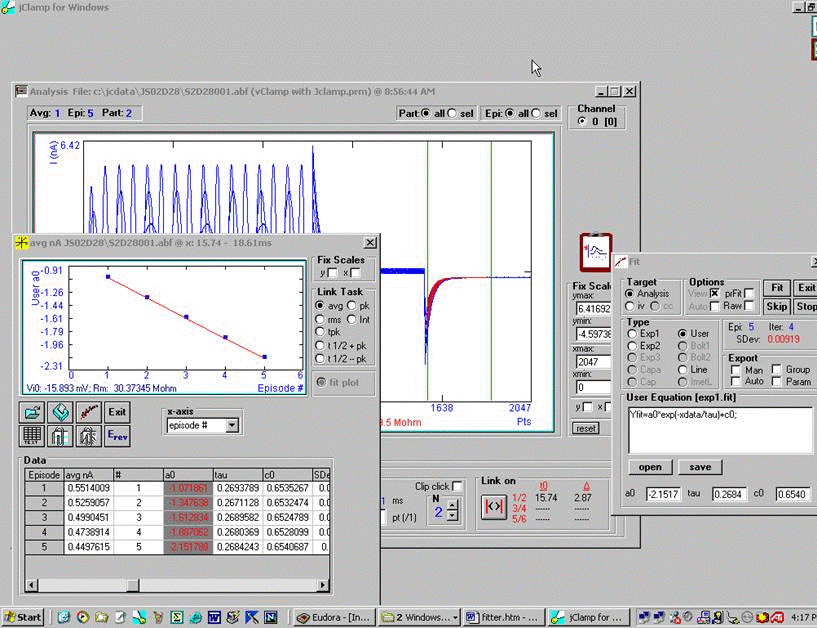
Fitting of data traces in each of the three graph windows (Analysis, CCdata, and IV – in the Fit window choose the desired target) can be made with built in and user defined equations using the Levenberg-Marquardt method. In the Analysis and CCdata window, the fitted region is between cursors 1 and 2. In the IV plot all data are fitted (but you can remove 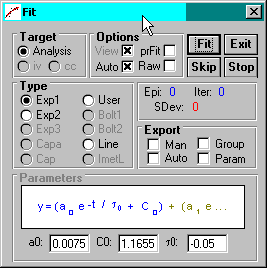 points by clicking on the data points in that graph). Built in functions will guess at initial parameters if the Auto check box is set. Uncheck it if you wish to provide your own guesses in the text boxes. Upon typing (actually upon key release) in any of the parameter text boxes, a trace in green is displayed to help with initial guesses. Remember that initial guesses are crucial for successful fitting! All traces displayed will be fitted. You should display only the traces that you want to fit.
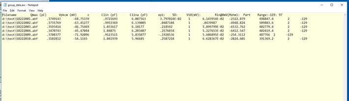
Data from the fits are sent to the Spreadsheet in the IV window (see image below). You may then plot the parameters vs any of the x-values in the IV window by clicking on the parameter column. Fitted parameters, original traces and fits can also be exported in tab-delimited ASCII format for importing into spreadsheets. Shift-click on Fit button will automatically copy data to clipboard for pasting. If the Man button is checked then you may choose the filename to save as or accept a default. If auto is checked then all subsequent fits are saved to the default filenames based on data filename. If group is selected then all data is save into a common group filename. If param is selected then only the parameters are saved. Sdev is the SD between real and fitted traces.
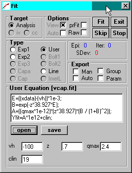
The user equations are placed in the user_fits directory under the jClamp32 directory. Use the open and save buttons to access the files. You can also simply write the equation in an ASCII editor and place in the user_fits directory. Each equation is housed in an ASCII file with the extension <.fit>. An example of a double exponential fit is given below. The format must be followed. The word xdata represents the x-values (in mV or ms) and the word Yfit must finally equate all previous equations. A semicolon must end all lines, and the headings ([equations] and [initial…) must be used. Most math functions are available. They are:
ABS, ACOS, ARCCOSINE, ACOSH, ATN, ATANH, SIN, SINH, COS, COSINE, COSH, TAN, TANH, EXP, LOG, SQR, LOG10
Make sure that non-parameter names are unique, since they will be used to place their equivalents within the final evaluated equation. For example, <ea> and <eb> below cannot be confused with any other part of the equation. But if you used an <da>, then all the <da>’s in the equation would be replaced with < a0*exp(-xdata/tau0)+c0> when I parse it.
----------------------------------------------------------------------
[equations]
ea=a0*exp(-xdata/tau0)+c0;
eb=a1*exp(-xdata/tau1)+c1;
Yfit=ea+eb;
[initial guesses for parameters]
a0=1.8549;
tau0=0.57;
c0=15.3114;
a1=2.1495;
tau1=2.7654;
c1=15.3114;
--------------------------------------------------------------------------------------
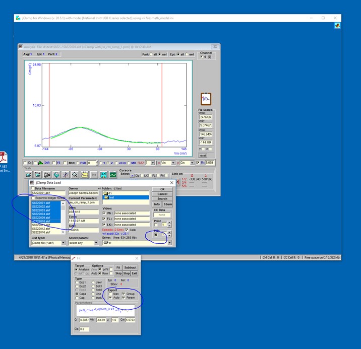
jClamp can do automatic group fits and save parameters automatically. Copy abf files with same protocol into a directory, and open one file. Set up fit to do, then check the boxes indicated below and choose multiple files then open. Data will be put in a group file in the directory.