Cm Analysis
Cell capacitance measurement in jClamp (www.scisoftco.com)
Cell capacitance measures are useful for a number of reasons. They can provide information on the surface area of cells, on the electrical coupling of cells, on the release or uptake of cellular vesicles, and on the voltage-sensor charge movement (gating currents) in the plasma membrane. In jClamp, a number of methods are available for capacitance measurement under voltage/current clamp, each having its own benefits.
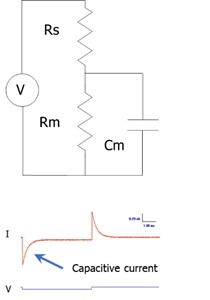
All estimates of cell capacitance are model dependent. The typical electrical model used is shown in the figure, where the voltage/current clamp system is defined with a driving source, a series resistance (Rs), membrane resistance (Rm) and a cell capacitance (Cm). This is the simplest model of a clamped cell. Stray capacitance resulting from amplifier, pipette holder and the pipette complicate the model. The typical model with stray capacitance, which can add frequency dependent interference into the simple model response, has a series combination of Cs and RCs in parallel with the source. Note that for the simple model, Cm is linear and thus frequency independent, providing electrical responses to driving forces which should produce estimates of Cm that are frequency independent. Obviously, stray capacitance can alter estimates of Cm that are derived from the simple model. In fact, Cm estimates that I discuss are derived from the simple model, and thus susceptible to stray capacitance interference. Stray capacitance effects must therefore be removed.
In your jClamp directory (/CM papers and tech notes) there are a number of files that are useful for understanding the following concepts and the issues that affect capacitance measurement capabilities. Take a look at them.
Time analysis
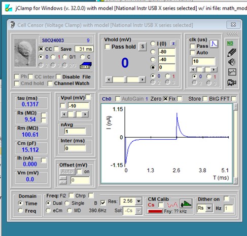
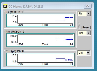
The most basic method to measure cell capacitance involves delivering a step voltage/current to the clamped cell. This is routine in jClamp and performed in the Cell Censor (CC) window. In voltage clamp, a small step voltage is delivered, and the currents are analyzed in the time domain to provide estimates of the circuit components using the approach in Huang and Santos-Sacchi, BJ, 1994 Appendix 1. A history window can display the values real time in a plot, and/or you can save the values for subsequent opening in the CC analysis window. See other sections of the help file to use these capabilities.
AC analysis
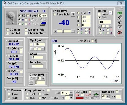
You can also do frequency domain cell parameter estimation. You may toggle between Time and Frequency mode on the fly. All selections in CC are enabled during CC data collection, for example, in Frequency mode you may change analysis type (Single , Dual, eCm, MD), or Sample Resolution, or holding potential or Vpul size on the fly. Place the mouse pointer over the values of Rs, Rm and Cm and a pop up shows the RMS value. Capacitance measures can also be made within ordinary protocols -- see Command Utility.CC Frequency domain analysis and protocol analysis work together to get clean Cm measurements. Below is a description of sine wave analysis in jClamp and more details about all features.
For all methods except dithering, it is imperative that you calibrate your system! Things will not work otherwise! See below for details on how to calibrate.
Single sine analysis
The current that is measured under voltage clamp is the current through Rs, namely IRs. In the single sine method a single sinusoidal voltage or current stimulus is delivered and the parameter values (Rs, Rm, Cm) of the patch/cell model (shown above) are estimated. This method of Cm estimation is based on evaluation of the changes of the capacitive current component of IRs, and arose from the initial work of Marty and Neher (1981), who tracked current at a phase angle that approximated the angle of ∂Y/∂Cm. This method was subsequently modified by Joshi and Fernandez (1988) to use the angle of ∂Y/∂Rs. See their paper for the reasoning behind this choice.
The method I employ here I devised by careful inspection of the phase tracking techniques above, and determination that the equivalent results are obtained by evaluating the imaginary component of IRs, B. Cm is estimated by using the gain factor (Hc) of 1/∂Y/∂Cm, which is approximated (Gillis, 1995) by
Hc = 1+ tan2 (90o–Y) ω-1,
where Y is the admittance at the angular frequency ω.
Cm= BHc .
A resistive measure (Rs) is estimated from the real component of Y, namely A, and scaled with abs(Y^2) Unlike typical phase tracking paradigms, a point-by-point analysis is performed. However, since the gain is approximated, the Cm estimate suffers from interference from resistive changes in the model, especially at low frequencies. This interference is alleviated by two additional methods that I have devised, the dual sine and eCm methods listed below.
Phase Sensitive Detector (PSD)
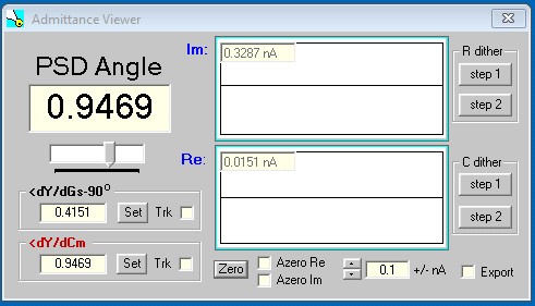
When single sine analysis is selected a check box is displayed which allows you to use the phase sensitive detector. The method is detailed by Gillis, 1995, but instead of integrating over a full cycle, I use the FFT to get at the real and imaginary component at any selected angle. Any angle can be chosen by moving the slider. Right clicking increments by 1.57 radians. The angle of ∂Y/∂Cm (derived from two sinusoids – see Santos-Sacchi, BJ, 2004) or the angle ∂Y/∂Gs – 90o can be set or toggled on for tracking. Zeroing and scale selection of the in phase (Y1) and quadrature (90o, Y2) response is possible. Pressing the left and right arrow keys will increment or decrement the PSD angle. You can use this see what angle is returned by dithering either the Rs or Cm amplifier compensation controls. The buttons on the right side implement angle estimation from dithering either the resistance or capacitance. Step one button is pressed to begin the process; then either RS compensation or Cm compensation controls need to be changed a small amount – no need to modulate the changes, just change a steady amount – then press step 2 button.
There is now a dither feature in the main CC window, which lets you repetitively dither Cm, Rs, or Rm when the math model is chosen or dither a digital pulse when hardware is turned on. The pulse could be used to dither Cm or Rs altering circuits. However, in the PSD mode there is a more simple dither technique to get at the right angle for Cm measurement which follows.
For Rs dithering, jClamp will calculate the angle at which currents are unchanged by Rs changes. For Cm dithering, jClamp will calculate the angle at which currents are unchanged by Cm changes.
Cm dithering is not really dithering the actual cell capacitance, so it is a rough estimate. Rs dithering will correct for changes in Rs, but Rm may change. Thus, obtaining an angle to measure true Cm is not possible with this type of dithering calibration. Using two sines, changes in all parameters can theoretically be separated. In any case, this traditional single sine approach can be used and if after obtaining an angle for Cm analysis you collect single sine data using a Command Utility protocol, the angle is saved with the data and can be used to analyze current magnitude at that angle and 90 degrees from it in the Analysis window. You might also use the digital out in a protocol to step a capacitance jump circuit in your patch clamp amplifier to roughly calibrate the Cm (Mag0 and Mag90) measurements.
Dual sine Analysis
In 1991, I devised a method to use two voltage sine waves simultaneously to enhance the parameter estimation method of Pusch and Neher (1988). A poster on the subject was presented at the Yale Neuroscience Retreat in 1992. Implementation of the technique to measure outer hair cell NLC at ms resolution was published subsequently (Santos-Sacchi et al., J. Phys., 1998).
The following description is taken verbatim from by funded NIH grant proposal (R01 DC02003, submitted in 1992).
…. In the present experiment, a discrete frequency analysis will be attempted. Pusch and Neher (1988) have used a single “tone” (sine wave, actually) technique to determine cell characteristics under whole cell voltage clamp. By injecting a sinusoidal voltage into a cell, and measuring the current response, they calculated from the system’s impedance, the cell capacitance, resistance and electrode resistance.
Rs=(A-b) / (A2 + B2 - A* b)
Rm=1/b* ((A-b)2 + B2) / (A2 + B2– A* b)
Cm=(1 / (ω * B))) ((A2 + B2– A* b)2 / ((A-b)2 + B2))
where,
b=1/(Rs+Rm)
Y=1 / Zin
A=Re(Y)
B=Im(Y)
ω=2 π f
As can be seen, with the use of one “tone” (ω), it is necessary to obtain an independent estimate of the input resistance (b). However, the utilization of a “two tone” (ω1 and ω2) stimulus allows one to determine all parameters, given the signal and response. That is, b need not be determined independently, and can be solved for, since, for example, Rs is the same at any two frequencies. The evaluations should work under voltage clamp or current clamp. …
The implementation in jClamp allows the use of several different time resolutions which depend on the selected clock. It is best to use the default settings, since only these have been checked to work effectively, but feel free to try different settings and verify with electrical models. Real and imaginary components of the current responses are obtained through Fast Fourier Transform. Remember the analysis is model dependent (see model above), although the technique has now been extended to fusion event (and junctional coupling) analysis – see help on Analysis.
jClamp now uses two approaches for 2 sine stimulation, one being the original implementation where f2=2*f1 (index into the FFT array being 1 and 2) – the Fi2 checkbox is unchecked, and the other f2<>f1*2 (index into the FFT being 2 and 3) – the Fi2 checkbox is checked. By making the latter stimulus we avoid possible two-tone distortions such as sums and difference frequencies that can be generated in a nonlinear system. Thus, for the original implementation, f1 of 390Hz and f2 of 781 Hz could generate distortion components at f2-f1 which would sum with the f1 response and potentially interfere with measurement of cell parameters. Other distortion components, e.g. harmonics, could also interact with the primary frequencies causing problems. Now I introduce a 2-sine signal that is immune from these effects. Since the indices are not harmonically related, distortion components of an f1 of 390Hz and f2 of 585Hz will not interact as before. The new implementation will provide a few differences from the old one. For example, the old implementation at 10 usec,would produce six resolutions at 0.16, 0.32, 0.64, 1.28, 2.56, 5.12 ms or correspondingly an f1 at ~ 6250, 3125, 1562, 781, 390, and 195 Hz, with f2 at 2*f1. On the other hand, the new implementation at 10 usec, will produce the same six time resolutions at 0.16, 0.32, 0.64, 1.28, 2.56, 5.12 ms but correspondingly f1 at ~12500, 6250, 3125, 1562, 781, and 390 Hz, and f2 at ~18750, 9375, 4687,2343,1171, and 585 Hz. Two cycles of f1 and 3 cycles of f2 are used for each measurement of cell parameters.
Detrending raw data
It is very important to detrend the data when sinusoidal stimulation is superimposed on rapidly changing voltage commands, as would be the case for investigation of voltage dependent capacitance using ramps. The method of detrending I use does not add significant additional noise to the analyzed data. When you check the detrend button during Cm analysis a widow pops up below the checkbox. The choices are auto and a range of numbers (detrending iterations) from 1-20. The auto feature chooses the correct number of detrend iterations, but there may be a number below that which has less noise in the Cm trace, so you can choose the number of iterations manually. Detrending removes rapidly changing currents (without filtering the 2-sine response) prior to FFT analysis. See the Detrending technical note supplied with jClamp.
eCm Analysis
This method estimates all parameters based on an exact solution of ∂Y/∂Cm and its angle. Though the method uses two sinusoids to get at the angle of ∂Y/∂Cm, all parameters are determined from inspection of only the low frequency response. The manuscript detailing this approach (Santos-Sacchi, Biophysical Journal, 2004) is in the jClamp directory.
Single sine analysis is performed on the lower frequency, f1. For command protocols, the number of frequencies can be set in the command window and is saved with protocols, so you can make and run either 2 sine or single sine commands.
Cm Analysis by Chirp stimulation (currently requires jClamp program authorization)
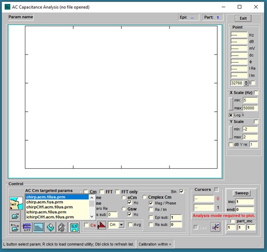
A chirp stimulus sweeps frequency across time and can be used to get frequency dependent information on Cm within a short stimulus period. This AC Cm mode is available to collect and analyze data. The AC Capacitance Analysis window can be opened from the Bar Menu or from the jClamp Analysis Window.
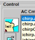
Files that use chirp stimulation intended for Cm measurement should be built in the Command Utility and saved with characters “.acm.” embedded in the protocol filename; for example, <my_test.acm.prm> or <my_othertest.acm.10us.prm>. Those parameter files will appear in the targeted param list within the AC Cm window (as well as accessible from the Command utility or RPD). Protocols must have the same clock as the loaded CM calibration file clock (see Calibration below). Click on one param and run the protocol by clicking on the large Init button.
After running a protocol or when abf data files of this type are opened they plot in the AC Cm Analysis windows. FFT requires continuous data to interrogate, so repeating chirps are built into each partition of a protocol; partitions at the start and end of a protocol should be avoided since discontinuities will be present in those responses. A few methods to analyze the data are available. These are 1) dual sine, 2) single sine (Rs correction must be made with this approach – enter in text box), 3) eCm, 4) Gsw (the last two methods can be adversely affected by noise in the data. Check the Hc checkbox to use magnitude calibration based on the true value of ∂Y/∂Cm or an estimate from Gillis, 1995). Move the mouse cursor over items in the window to get some information shown in the bottom panel or tooltip text. The final method is 5) complex capacitance, where AC currents at 0 and 90 degrees phase re voltage phase are analyzed to provide real and imaginary (or magnitude and phase) components of Cm. For us, we use this approach to measure the frequency response of NLC (prestin voltage-sensor/gating charge movement). In the figure below, NLC complex capacitance is extracted from a macro-patch on the OHC lateral membrane and shows low pass behavior in the real (or magnitude) component. From the Analysis plot, further analysis can be
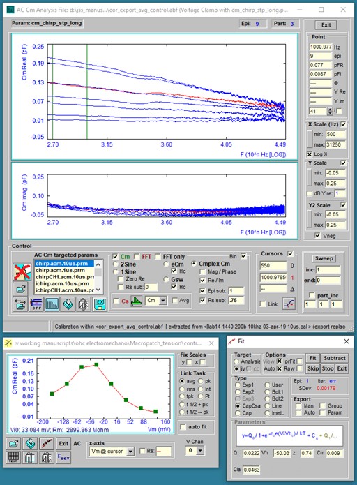
made using “IV” plots of the capacitance data. For example, the IV Plot Window plots the cursor selected trace magnitudes at 1000.977 Hz versus step voltage where chirps were superimposed and fits the data to a derivative of a Boltzmann function (NLC).
System Calibration for Cm Analysis-- read this whole section!
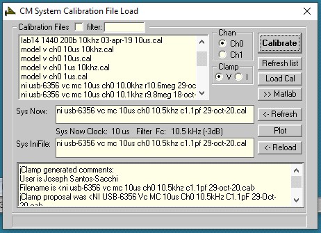
In order to make accurate AC measures of membrane capacitance, admittance data from raw currents needs to be corrected for the frequency response of the system. Calibration can be initiated by clicking the ruler icon in CC. When pressed, a window appears that allows you to either load an existing calibration file, or run a calibration protocol. Upon calibration the ruler icon turns green. Any changes in the stimulus settings which alter the system response will require a new calibration file. This includes changes to the clock or external filters. Filters should be set to a cutoff frequency (Fc) less (about half is good) than the displayed Nyquist frequency (Fny) indicated for a given clock. Calibrations can be loaded from disk (file named filename.cal) using the file command buttons.
Calibration depends on the pure resistivity of the calibration resistor, or in the case of the dither technique, the pure resistivity of the whole dithering unit. Unfortunately, stray capacitance and inductance accompanies these components. For dual sine measures in CC and Command Protocols, I find it best to work with low frequency stimulation, sine 1 at @ 390 Hz and sine 2 @ 781 Hz, the default setting at a clock of 10 us. In any case, you should always check the reliability of the measures with an electrical cell model!
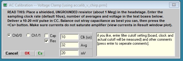
One method for calibration is to use a resistor between head-stage and ground. The lower the value the better, since less stray capacitance will accompany the resistor – i.e., it will more reflect a true resistance. A value of 1 Mohm is a good compromise. During calibration, a window opens (see below) to allow selection of channel, clock and voltage. The protocol file <accalib_v_chirp.prm> (or <accalib_i_chirp.prm> for current clamp) is used for calibration and is run automatically during calibration. The voltage magnitude, in the protocol can be increased as long as saturation is not evidenced in the current response. The protocol generates a correction file for the real and imaginary components of the system. Remember, the resultant calibration file has calibration data for a given amplifier, A/D, clock and filter cutoff; again, if any change another calibration file is necessary. During measurement of cell capacitance the voltage magnitude should be as small as possible to implement small signal analysis that tends to eliminate nonlinearities (I typically use 10 mV peak). See Takahashi S, Santos-Sacchi J, Distortion component analysis of outer hair cell motility-related gating charge., J Membrane Biol 169: (3) 199-207, 1999 for potential problems with the technique. A non-harmonic protocol now implemented in jClamp can overcome these distortion problems if you have significant distortion. See description of the non-harmonic technique above.
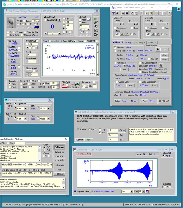
The Calibration procedure is described below. I have devised a new way to get around some problems with stray capacitance, which heretofore had to be removed fully (if possible) by compensation at the amplifier. Now, although it is best to balance out stray capacitance as best you can to limit potential saturation of the amplifier, jClamp can remove stray capacitance during calibration and prior to cell recording. For voltage clamp you may make a calibration file using either a resistor or capacitor; thus, the following window appears after pressing the Calibrate button. Follow instructions in the Windows.
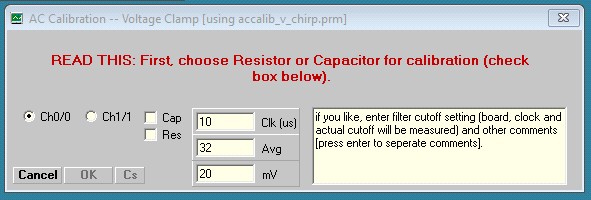
Here we have chosen a resistor to use. After balancing out stray capacitance, in this case with the auto compensation feature in Axon Multiclamp 700B commander window, the following result shown below is obtained. Note that in the CC Window the trace is simply a noisy flat line without capacitive spikes at onset and offset. Despite what looks like perfect stray capacitance cancellation, the chirp response shows a high frequency current response in the lower Result plot.
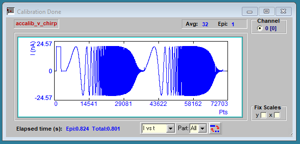
jClamp will removed that uncompensated response to get at the true system response which is obtained after grounding the resistor and pressing the OK button. The response now is plotted below, and you are asked to save the calibration file with a suggested filename. You can save it with a different filename, but jClamp stores the suggestion as information which shows in the CM System Calibration File Load window.
If the Cap check box is checked to use a capacitor for calibration, follow instructions in the widows, as you did above.
For current clamp the procedure differs, and an alternate window will appear – you must compensate capacitance before calibration. The current clamp calibration window will open if CC is set in current clamp mode, else it will open for voltage clamp calibration.
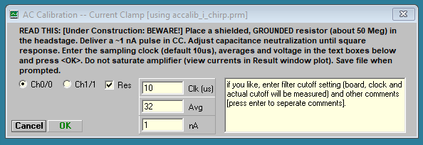
In current clamp mode the resistor should be grounded and the voltage response to a short current pulse should be squared by using the amplifier capacitance neutralization. Then calibrate by pressing OK button. Current clamp calibration and Cm measurement are still under development. Beware!
Save the calibration data file and it is loaded as the default system calibration. Note that it can be reloaded (as default set in the ini file or loaded with CC window access to CM Calibration Load window). It should be used only when the system (i.e., clock and filter settings in CC) and protocols match the original calibration settings. Remember, voltage and current clamp frequency responses within the same amplifier unit may differ, so each may require using unique calibration files.
Each channel must be calibrated if you want to use them. The channel is selected in the calibration window. When you calibrate, channel 0 is defined as channel 0 out with channel 0 in, and channel 1 is defined as channel 1 out with channel 1 in. Check the goodness of the calibration with an electrical model. You will need to balance out the model series resistance's stray capacitance first which you can do under whole cell conditions using the MD/Cs method – see below. The default capacitance calibration files (vClamp and iClamp) are set in the ini file of your choice.
Here is an important point to remember. The Cm determination is model dependent and assumes no stray pipette capacitance. This is also true when you use an electrical model cell. If you have a commercial cell model, typically you cannot really balance out the stray capacitance of the series resistance under whole cell conditions. However, this can be done suing the MD/Cs method below. To confirm proper calibration and stray capacitance removal, you should make a simple cell model in which you can manually disconnect the series resistance from the cell’s parallel resistance and capacitance. Balance out the series resistance stray capacitance when it is disconnectedinto the air as you do during calibration. Then connect the rest of the model and the measured values will be quite accurate and should match those you obtain with the MD/Cs method.
For command protocol data collections, the system calibration file is saved with the <abf > data file and is automatically used for correction in analyses. So, <abf> data files are saved raw and analyzed each time the file is opened. This means that for any <abf> file, different calibration files can be used to analyze the data. If you had collected data mistakenly with the wrong system calibration file, you may load a correct calibration file when in Analysis mode, and even export that data with the correct calibration.
Finally, be careful to understand how you might interfere with valid correction using a given calibration. The calibration simply “flattens” out an “unflat” system response; it removes the system response from the equation so you can accurately gauge the cell’s physiological response. Let’s review the calibration procedure. When you place a pure resister between headstage and ground (and balance out the stray capacitance), the response that you measure which deviates from a purely resistive response should be due to the amplifier, filter, D/A characteristics and any other influential component that you have in the path between that resister and the recorded response. If everything is done correctly with the calibration (pure resistivity, etc.) then we get correction factors (for all frequencies at the given clock rate) that can be used to remove the effect of the equipment, and thus measure the cell’s admittance correctly. In order to validly use the correction factors, you have to make sure that after the formation of a gigohm seal, stray capacitance is balanced out (but see MD/Cs method below) because the evaluation of the cell’s characteristics is model dependent and does not include a pipette capacitance. Additionally, any manipulation of the amplifier after whole cell configuration could potentially introduce changes to the state of the system that could invalidate the calibration. For example, series resistance compensation may involve (in some amplifiers) an introduction of a lag in the system. This could invalidate the correction values in the calibration file. You can check the effect of series resistance compensation or other amplifier manipulations with an electrical model cell. I routinely will not use this feature if I am doing capacitance measures. The best thing that I can say is that you should check everything you might do with a model cell before trying on a real cell.
In-cell stray capacitance neutralization with software assistance
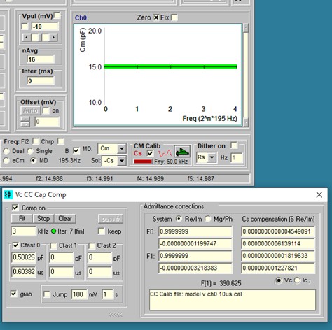
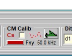
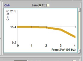
Although you may have made efforts to remove stray electrode capacitance prior to popping into a cell, things may change during the course of an experiment. For example, fluid level may rise or fall around the electrode and additional stray capacitance may interfere with Cm measures. I now provide simultaneous multi dual (MD) sine wave analysis to handle this problem. In CC, select the MD checkbox and 5 dual f1/f2 frequency analyses will provide a plot of Cm versus frequency index (low f to high f). If the line is not flat then stray capacitance probably is present. Simply flatten the line with electrode capacitance compensation circuitry on the patch amplifier to correct for stray capacitance at all frequencies. Color of the line changes towards green as the correct compensation is reached (see last figure). An accurate calibration file is essential to use this feature. With this technique, you need not worry if you pop into a cell before adequately compensating stray capacitance. It must be emphasized that this procedure demands that cell capacitance must be linear, i.e., surface area dependent only. If a nonlinear capacitance exists, this must be performed in a state where it is absent.
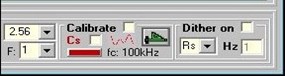
A Capacitance Compensation window is now available to aid in stray capacitance (Cs) compensation. It is opened by checking the Cs checkbox in the CC window in Calibrate sub frame. Some amplifiers (e.g. Axon Multiclamp) may not have enough compensation to flatten out the Cm vs F curve in MD. Additional compensation is provided by moving the mouse with the left button pressed when over the text boxes. Finer control is afforded by the mouse wheel scroll alone. Right click on text box to set 0.1, 1.0 and 10X gain changes. One could do all compensation with the software controls but it is better to balance fully with hardware if possible. This software compensation works only under Frequency domain, but hardware compensation works under all stimulation conditions since it is at the amplifier. One could compensate Cs in Freq domain and switch back to Time domain knowing that the compensation remains in effect. It is really impossible to balance out stray capacitance under the Time domain when inside the cell, thus the MD/Cs method is very useful even if you do not do Cm measurements.
Under some conditions, it may be possible to compensate automatically in software. First adjust hardware compensation just below compensation as shown in the red line below. Then press the fit button. The success of this depends on many factors, including the initial guess result prior to minimizing to a slope of Cm vs F of zero. Now jClamp gets an initial guess for Cs magnitude from a 4 parameter fit of the model with only a Cs (+ Rs, Rm, Cm), and no Rcs. This quick accurate estimate allows fitting to be done very quickly.
For the Multiclamp and EPC10, fitted paramaters can be sent to the patch clamp directly. Additionally, for the Multiclamp, checking the MC box will fit the parameters solely in MC Commander. If the passed fit is not accurate, hit <Alt> to show a button [C] that will calibrate the transfer of jClamp fitted parameters to Multiclamp. MD mode must be in effect.
The One last note, the Cs corrections are saved with the data file and utilized during analysis – there is a Cs checkbox in the Analysis window which enables/disable the corrections so that you can see the effect of having successful stray Cs compensation. Each new cell must be compensated, and probably during an experiment with one cell you should check compensation. The actual voltage delivered to the cell during MD stimulation is larger than a 2 sine stimulus because 5 sines of equal magnitude are summed. Thus, you may want to consider the effect of the stimulus on your cell. If necessary, you could reduce the stimulus size during compensation.